Electrode Creation

Before creating any electrodes, we need to familiarize ourselves with a few concepts. First- whenever you initialize a system, you need to pick nr, nz, axial_size and radial_size. nr is the grid resolution in the r-dimension, and nz is the same for the z-dimension. Axial_size is the total length of the domain in meters in the z-dimension, and radial_size is the same for the r-dimension.

This means the grid resolution in the z-dimension is axial_size/nz, and in the r-dimension is radial_size/nr. You should, if using nonstandard values for these, ensure you’re aware of these so you can properly convert from grid units to meters.

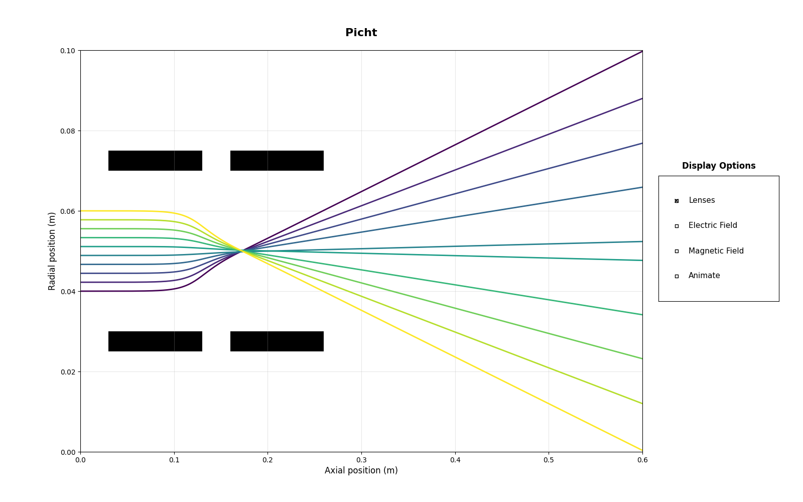
You can initialize a two-cylinder lens with -5000V and 0V respectively as follows:

import numpy as np
from picht import ElectronOptics, ElectrodeConfig
import matplotlib.pyplot as plt

system = ElectronOptics(nr=100, nz=600, axial_size=0.6, radial_size = 0.1)

electrode = ElectrodeConfig(
    start=30,
    width=100,
    ap_start=30,
    ap_width=40,
    outer_diameter = 50,
    voltage=-5000
)

system.add_electrode(electrode)
electrode1 = ElectrodeConfig(
    start=160,
    width=100,
    ap_start=30,
    ap_width=40,
    outer_diameter = 50,
    voltage=0
)

system.add_electrode(electrode1)

potential = system.solve_fields()

trajectories = system.simulate_beam(
    energy_eV= 1000,
    start_z=0,
    r_range=(0.04, 0.06),
    angle_range=(0, 0),
    num_particles=10,
    simulation_time=2e-8
)

figure = system.visualize_system(
    trajectories=trajectories,
    display_options=[True, False, False, False]) #only switches on the lens visualization, keeps the e-field, b-field and animations off in the start, so the generated thumbnails look cleaner

plt.show()